Monday, October 12, 2015

NESTED IF Condition

How to use the IF statement in Excel when you had two conditions that had to be met. For example, when sales fell between a 
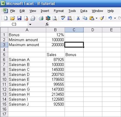
minimum and maximum number. Let’s take a look at our example again. Note that I’ve added the maximum amount of $200K into cell B3:
Before we go further, if you’d like to work through the examples yourself, here’s the raw data you can copy into an Excel worksheet. First, open up a blank excel worksheet. Next, highlight the table below. Copy it, and then go back to your excel worksheet. Go to cell A1 (or another empty cell, if you want to put the data elsewhere), and then select “Edit” from the menu bar. Select “Paste Special” and then “Text” from the popup box. Click “OK”. The data should appear in your Excel worksheet just as it does above.
Bonus 12%
Minimum amount 100000
Maximum amount 200000

Sales Bonus
Salesman A 87925
Salesman B 100000
Salesman C 145000
Salesman D 200750
Salesman E 178650
Salesman F 99555
Salesman G 147000
Salesman H 213450
Salesman I 122680
Salesman J 92500
Ok,,,,
Now, let’s suppose sales have to be greater than or equal to $100K and less than $200K for a salesman to receive a 12% commission rather than just be greater than $100K, as in our introductory example. How would you write that in “Excel-speak”?

It turns out that you can use Excel’s AND function, which Excel calls a logical operator (just like it calls the IF function). And, as usual, unlike how most other programming languages work, the syntax required in Excel is a bit different. To use it correctly, you have to write it like the following:
=AND(first condition, second condition, …, etc.)
(In other programming languages, AND would fall in between each condition, just like how we normally talk, but not in Excel!)
Let’s go back to the concrete example. To write the condition that sales have to fall betwen $100K and $200K for the salesman to receive a 12% commission, we’d write the following in cell C6:
=IF(AND(B6>=$B$2, B6<$B$3),B6*$B$1,"No bonus")
Like this:

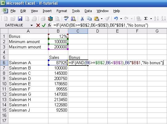
Translated into plain English, our IF statement now reads, “If B6 is greater than or equal to B2 and B6 is less than B3, then multiply B6 by B1. If not, then put ‘No bonus’ into the cell.” In the first case, our salesman didn’t meet the $100K requirement, so the AND function returned a false, so the IF statement put “No bonus” into the cell. By the way, in our case, we only had two conditions to meet, but if we had more, we could just keep adding them into the list of conditions in the parenthese after the AND function.

Saturday, October 10, 2015

VLOOKUP function

VLOOKUP function


Use VLOOKUP, one of the lookup and reference functions, when you need to find things in a table or a range by row. For example, look up an employee's last name by her employee number, or find her phone number by looking up her last name (just like a telephone book).
The secret to VLOOKUP is to organize your data so that the value you look up (employee’s last name) is to the left of the return value you want to find (employee’s phone number).

Syntax

VLOOKUP (lookup_value, table_array, col_index_num, [range_lookup])
For example:
  • =VLOOKUP(105,A2:C7,2,TRUE)
  • =VLOOKUP("Fontana",B2:E7,2,FALSE)
Argument name Description
lookup_value    (required) The value you want to look up. The value you want to look up must be in the first column of the range of cells you specify in table-array .
For example, if table-array spans cells B2:D7, then your lookup_value must be in column B. See the graphic below. Lookup_value can be a value or a reference to a cell.
table_array    (required) The range of cells in which the VLOOKUP will search for the lookup_value and the return value.
The first column in the cell range must contain the lookup_value (for example, Last Name in the picture below.) The cell range also needs to include the return value (for example, First Name in the graphic below) you want to find.
Learn how to select ranges in a worksheet.
col_index_num    (required) The column number (starting with 1 for the left-most column of table-array) that contains the return value.
range_lookup   (optional) A logical value that specifies whether you want VLOOKUP to find an exact match or an approximate match:
  • TRUE assumes the first column in the table is sorted either numerically or alphabetically, and will then search for the closest value. This is the default method if you don't specify one.
  • FALSE searches for the exact value in the first column.
The following picture shows how you'd set up your worksheet with =VLOOKUP("Akers",B2:D5,2,FALSE) to return Kim.
Example of value and array needed to create a VLOOKUP formula in Excel

Examples

To use these examples in Excel, copy the data in the table below, and paste it in cell A1 of a new worksheet.
ID Last name First name Title Birth date
101 Davis Sara Sales Rep. 12/8/1968
102 Fontana Olivier V.P. of Sales 2/19/1952
103 Leal Karina Sales Rep. 8/30/1963
104 Patten Michael Sales Rep. 9/19/1958
105 Burke Brian Sales Mgr. 3/4/1955
106 Sousa Luis Sales Rep. 7/2/1963
Formula Description
=VLOOKUP("Fontana",B2:E7,2,FALSE) Looks for the value Fontana in the first column (column B) of table_array B2:E7 and returns the value Olivier found in the second column (Column C) of the table_array. The range_lookup FALSE returns an exact match.
=VLOOKUP(102,A2:C7,2,FALSE) Searches for an exact match of the last name for lookup_value102 in column A. Fontana is returned. If lookup_value is 105, Burke is returned.
=IF(VLOOKUP(103,A1:E7,2,FALSE)="Sousa","Located","Not found") Checks to see if the last name of Employee with ID 103 is Sousa. Because 103 is actually Leal, the result is Not found. If you change "Sousa" to "Leal" in the formula, the result is Located.
=INT(YEARFRAC(DATE(2014,6,30), VLOOKUP(105,A2:E7,5, FALSE), 1)) For the fiscal year 2014, finds the age of the employee with ID 105. Uses the YEARFRAC function to subtract the birth date from the fiscal year end date and displays the result 59 as an integer using the INT function.
=IF(ISNA(VLOOKUP(105,A2:E7,2,FALSE)) = TRUE, "Employee not found", VLOOKUP(105,A2:E7,2,FALSE)) If there is an employee with ID 105, displays the employee's last name, which is Burke. Otherwise, displays the message Employee not found. The ISNA function (see IS functions) returns a TRUE value when the VLOOKUP function returns the #N/A error value.
=VLOOKUP(104,A2:E7,3,FALSE) & " " & VLOOKUP(104,A2:E7,2,FALSE) & " is a " & VLOOKUP(104,A2:E7,4,FALSE) For the employee with ID 104, concatenates (combines) the values of three cells into the complete sentence Michael Patten is a Sales Rep.

Common Problems

Problem What went wrong
Wrong value returned If range_lookup is TRUE or left out, the first column needs to be sorted alphabetically or numerically. If the first column isn't sorted, the return value might be something you don't expect. Either sort the first column, or use FALSE for an exact match.
#N/A in cell
  • If range_lookup is TRUE, then if the value in the lookup_value is smaller than the smallest value in the first column of the table_array, you'll get the #N/A error value.
  • If range_lookup is FALSE, the #N/A error value indicates that the exact number isn't found.
Learn more about errors in worksheets, like #N/A, #REF, and the rest.
#REF! in cell If col_index_num is greater than the number of columns in table-array, you'll get the #REF! error value.
#VALUE! in cell If the table_array is less than 1, you'll get the #VALUE! error value.
#NAME? in cell The #NAME? error value usually means that the formula is missing quotes. To look up a person's name, make sure you use quotes around the name in the formula. For example, enter the name as "Fontana" in =VLOOKUP("Fontana",B2:E7,2,FALSE).

Best practices

Do this Why
Use absolute references for range_lookup Using absolute references allows you to fill-down a formula so that it always looks at the same exact lookup range.
Learn how to use absolute cell references.
Don't store number or date values as text. When searching number or date values, be sure the data in the first column of table_array isn't stored as text values. Otherwise, VLOOKUP might return an incorrect or unexpected value.
Sort the first column Sort the first column of the table_array before using VLOOKUP when range_lookup is TRUE.
Use wildcard characters If range_lookup is FALSE and lookup_value is text, you can use the wildcard characters—the question mark (?) and asterisk (*)—in lookup_value. A question mark matches any single character. An asterisk matches any sequence of characters. If you want to find an actual question mark or asterisk, type a tilde (~) in front of the character.
For example, =VLOOKUP("Fontan?",B2:E7,2,FALSE) will search for all instances of Fontana with a last letter that could vary.
Make sure your data doesn't contain erroneous characters. When searching text values in the first column, make sure the data in the first column doesn't have leading spaces, trailing spaces, inconsistent use of straight ( ' or " ) and curly ( ‘ or “) quotation marks, or nonprinting characters. In these cases, VLOOKUP might return an unexpected value.
To get accurate results, try using the CLEAN function or the TRIM function to remove trailing spaces after table values in a cell.